Backpropagation: The Algorithm That Underpins Neural Networks

Backpropagation in simple terms

Definition: Backpropagation efficiently computes the gradient of a neural network's loss function with respect to its weights and biases using the chain rule, enabling iterative optimization through gradient descent.

What does this mean?: During training, a neural network ingests some batch of training data and returns a batch of predicted outputs. The difference between the predicted outputs and correct outputs is computed (loss) to see how far off the neural network is from where it should be.

Backpropagation enables the neural network to know which direction (gradient) to tweak each of its parameters (weights and biases), to minimize its loss. All the parameters are nudged in the direction corresponding to their gradients (this is called gradient descent) until the training run is complete. At the end of a successful training run, all gradients will be near zero, indicating that nudging the parameters any more will not improve the accuracy of the neural network.

The chain rule mathematically ensures that the gradient of every parameter can be calculated from just the loss, as long as all functions in the neural network are differentiable (i.e. the function is continuous and smooth).

Without backpropagation, the neural network will not know which direction to nudge its parameters. At worst case, it will need to try every combination of parameter values to tune itself, which is computationally infeasible for any large neural network.

Below, we explore what is a neural network, then study the math of backpropagation.

What is a neural network

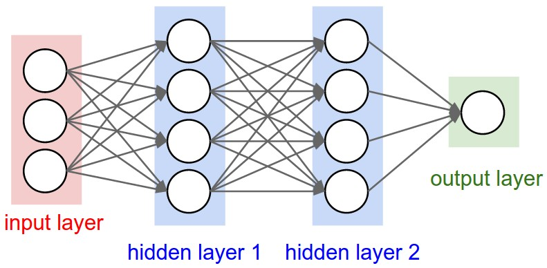
A neural network is made up of layers of neurons which are interconnected to each other. Each neuron takes numbers, from the input layer or neurons in the previous layer, and performs arithmetic on it, then passes it to a neuron in the next layer. A common neural network structure is that of a multi-layer perceptron (MLP), which consists of:

• Input Layer:

  • Accepts the raw data into the network (e.g., images, text, or numerical data).
  • Each neuron in this layer represents one feature of the input.

• Hidden Layers:

  • Perform intermediate computations to extract patterns or features.
  • Consist of neurons connected to the previous and next layers, with weights determining the strength of each connection.

• Output Layer:

  • Produces the final prediction or decision, such as a classification label or a numerical value.

Each hidden layer in a neural network can be thought of as a sort of neuron cell which accepts an axon (x), multiplies it by a weight (W), adds these weighted axon values together, adds a bias (b), then passes it through an activation function f(∑wx+b), which outputs it to the next layer of the neural network.

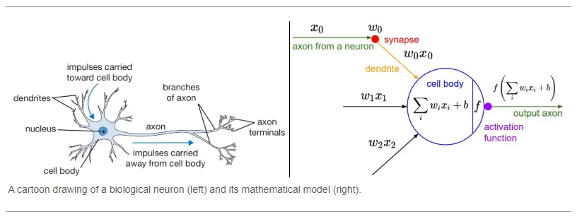
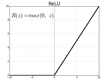
An activation function is a function that determines whether a neuron should be activated, i.e. whether its value should be passed onto the next layer. It introduces non-linearity to the network, enabling it to learn complex patterns in the data. A commonly used activation function is Rectified Linear Unit (ReLU), which simply passes on the input if it is positive, and makes it zero if it is negative.

Forward propagation

Neural networks undergo several iterations of forward propagation, loss calculation, and backpropagation as they ingest batches of training data to tune the neural network weights.

During forward propagation, the neural network takes the input training data and passes it through each layer to output a result.

Forward propagation example:

This MLP tries to predict how hours of studying (x1) and hours of sleep (x2) predict exam pass/fail (y):

• Input Layer: 2 neurons
  • Takes the input features x1 (hours of studying), and x2 (hours of sleep)
• Hidden Layer: 3 neurons
  • Each neuron calculates z = W ⋅ X + b, where W is the weight, X = [x1, x2], and b is the bias
  • A ReLU activation function is applied: a = max(0,z)
  • Outputs a₁, a₂, a₃ as the activations from the 3 hidden neurons
• Output Layer: 1 neuron (y)
  • Takes inputs a₁, a₂, a₃ and calculates z_out = W_out ⋅ A + b_out, where A = [a₁, a₂, a₃]
  • Applies a sigmoid function to produce y_pred = σ(z_out), the predicted probability of passing

Loss calculation

The network compares its predictions to the true labels (targets) using a loss function to measure how well it performed.

Aside: in unsupervised learning where there are no true labels, loss may be calculated by how well the network clusters similar data points together, e.g. k-means loss.

Loss calculation example:

A function calculates how far off the prediction is from the target contained in the training data using mean squared error (MSE), where Y is the target, Ŷ is the prediction, and n is the training batch.

Aside: a better loss calculation for this task is binary cross entropy loss, but this is not necessary to understand backpropagation. Here is a good resource explaining binary cross entropy loss.

During backpropagation, we ask: in order to minimize the loss, what direction (gradient) does each weight and bias in the neural network need to move in?

Backpropagation

The network adjusts the weights and biases by propagating the error (loss) backward through the network. This is done using gradients computed via the chain rule in calculus.

Gradient
Recall from calculus that the slope of a curve at some point is its rate of change. The gradient is the slope of a multi-dimensional curve at some point. A more formal definition can be found here. During backpropagation, we are trying to find the gradient of every single paramater in the neural network. By finding the gradient of all parameters, we know which direction to nudge all parameters before the next iteration of forward propagation.

Chain rule
The chain rule is the most important mathematical principle in neural networks because it enables backpropagation to be computed. The chain rule states that the derivative of a composite function (dz/dx) is calculated by multiplying the derivative of the outer function (dz/dy) with the derivative of the inner function (dy/dx):

What this means is, as long as every neuron in the network uses a differentiable function (wx+b and the activation function ReLU are both differentiable), we can calculate the gradient (slope) associated with every single weight and bias in the neural network. We start with the neurons connecting to the output neuron and work our way back to the input neurons.

Backpropagation example:

Gradients of the loss function with respect to all weights and biases are computed using the chain rule of differentiation.

• Output Layer:

  • Error at the output neuron:
    δ_out = y_pred - y
  • Gradients for weights and biases in the output layer:
    ∂_Loss / ∂W_out = δ_out ⋅ A
    ∂_Loss / ∂b_out = δ_out

• Hidden Layer:

  • Error at each hidden neuron:
    δ_hidden,i = δ_out ⋅ W_out,i ⋅ ReLU'(z_i)
    where ReLU'(z_i) = 1 if z_i > 0, else 0.
  • Gradients for weights and biases in the hidden layer:
    ∂_Loss / ∂W_i = δ_hidden,i ⋅ X
    ∂_Loss / ∂b_i = δ_hidden,i

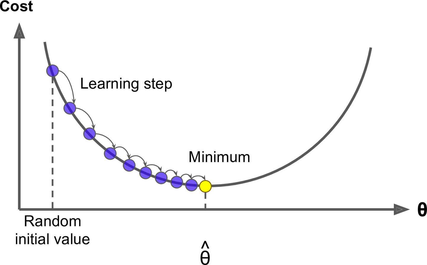
Once the gradient of every parameter (weights and biases) is calculated, the gradient is multiplied by a pre-determined step (such as 0.001) and the neural network starts another iteration of forward propagation, loss calculation, and backpropagation.

Summary

To summarize, forward and backpropagation essentially does gradient descent over a multi-dimensional, non-convex loss surface:

1. During forward propagation, the input data is passed through the network, applying weighted sums, biases, and activation functions at each layer
2. The computed loss defines a point on the high-dimensional loss surface
3. Backpropagation determines the direction and magnitude of the steepest descent on the loss surface
4. Gradient descent updates the network's weights and biases by taking a step in the direction of the negative gradient

The key mathematical principle which enables gradient descent is the chain rule which states that you can determine the partial derivative of z wrt x by calculating the intermediate derivatives: z wrt y, and y wrt x. This allows the gradient calculation to be propagated backwards, starting with the output and ending with the weights connecting the input layer to the first hidden layer (hence the term backpropagation).

Resources:

• Build a NN and implement backpropagation from scratch by Andrej Karpathy: https://www.youtube.com/watch?v=VMj-3S1tku0
• Slides from CS231n Deep Learning for Computer Vision by Stanford: https://cs231n.stanford.edu/slides/2024/lecture_4.pdf
• Learning Internal Representations by Error Propagation by Geoffrey Hinton: https://stanford.edu/~jlmcc/papers/PDP/Volume 1/Chap8_PDP86.pdf